What You Will Do:

• Draw your prediction of how light intensity changes as you move the MotionCart farther from a light source.
• Collect light intensity data in the Desmos Graphing Calculator by rolling the MotionCart away from your phone lamp.
• Compare function families (linear, polynomial, power, rational, exponential decay) and use sliders to decide which family best models the relationship between distance and light intensity.
• Complete the Google Docs worksheet and submit it according to your teacher's instructions.

Getting Ready:

• Light intensity: a measure of how much light energy reaches a surface, commonly measured in lux (lx).
• Position: how far the cart has moved from its zero position, measured in centimeters (cm). In this activity, position represents the distance between the light source (zero position) and the MotionCart's light sensor.
• Linear function: a function that changes at a constant rate. The graph is a straight line.
  $$y = mx + b$$
• Polynomial function: a function built from powers of the variable combined with constants.
  $$y = ax^{2} + bx + c$$

• Power function: a nonlinear function that involves a variable raised to a constant exponent. Negative exponents produce decreasing curves, while positive exponents create increasing curves.
  $$y = ax^{p} + b$$
• Rational function: a function with the variable in the denominator. Rational functions can show steep decreases and asymptotic behavior.
  $$y = \frac{m_2}{(x + b_2)^{2}}$$
• Exponential decay function: a function in which y-values decrease by a constant multiplicative factor for equal changes in x. The graph approaches a horizontal asymptote.
  $$y = ae^{kx} + b, \quad k < 0$$
• Interpolation of a model: using the graph of a mathematical model to estimate an intensity value for a distance that lies between the real data points.
• Extrapolation of a model: extending the pattern of the model to estimate intensity for distances beyond the range of the real data.
• Mathematical model: an equation or graph used to represent a real-world relationship between variables so that predictions can be made from the pattern.
• Click this link MotionCart - Activity 4 to open the worksheet in a new browser tab. Click Make a copy to save your version to your Google Drive.

What is Going On?

• Your phone lamp emits light outward in all directions from a single point. As the MotionCart rolls away, that light spreads over a larger and larger region of space, so the sensor receives less of it. In this activity you are tasked with finding which mathematical function models that relationship best.
• To better understand the phenomenon, imagine the light expanding outward from your phone like the surface of a balloon being inflated. The surface area of a sphere with radius $r$ is:
  $$A = 4\pi r^{2}$$
  As $r$(distance from phone) increases, the light energy is dilutted over a larger and larger surface area (A) and becomes dimmer. The 3D Desmos graph below shows this expanding sphere in real-time as you roll the cart.
• The four function families in the Desmos graph below each make a different prediction about how intensity and distance are related. A linear model assumes a steady, constant rate of change. A polynomial model allows for curvature driven by a squared or higher-power term. A power model lets the exponent be any constant, including fractions or negatives, producing a wide variety of curve shapes. A rational model places the distance variable in the denominator, producing a curve that drops steeply and levels off. An exponential decay model decreases by a constant multiplicative factor for each equal step in distance.
• Each model has adjustable parameters (sliders) that let you shift, stretch, or reshape the curve. Your job, after you have collected distance vs. intensity data, is to adjust those sliders and judge - based on how closely each curve follows your actual data points across the full range of distances - which function family gives the most convincing description of what you measured.

Explore the Geometry:

• The sphere shows how light spreads from your phone lamp: its radius tracks the cart's distance in real time, and its brightness is the cart's live light sensor reading.
• Follow these steps, the same as in the Getting Started with MotionCart activity, to connect your cart and observe the geometry of the phenomenon in the simulation before collecting data:
  1. Press and hold the button on the MotionCart for one second. The blue LED will blink, showing the cart is ready to connect.
  2. Click Connect Cart in the top bar. Select your MotionCart from the pop-up and click Pair.
  3. Once connected, the blue LED turns solid and Status changes to Measuring. Live Position and Light readings will appear in the top bar.
  4. Clear about one meter of desk space to roll the cart freely. Dim the surrounding light in the room and position your computer screen so it does not shine on the cart's light sensor.
  5. Turn on your phone's flashlight. This should be the main light source shining on the sensor. Prop the phone at one side of the clear desk area.
  6. Place the MotionCart approximately 10 cm from the phone flashlight with its light sensor (the cart's front face, just below the USB-C port) facing it. Starting at 10 cm avoids the saturation zone immediately next to the lamp where the sensor reading is unreliable. Click Zero Position - the sphere should shrink to its smallest size and Position should read 0.
  7. Slowly roll the cart away from the lamp and watch the sphere. The radius should increase and the patch should dim as you move farther away. If the radius decreases instead, click Change Sign to reverse the direction, then roll the cart away again to confirm the sphere grows as distance increases.
  8. Roll the cart back and forth a few times to explore how the sphere responds. Once the simulation looks correct - radius growing and patch dimming as you roll away - you are ready to collect data.

What Do You Think?

1. Based on your observations of the sphere simulation, use your mouse to click and drag on the graph below to draw your prediction of how light intensity changes as the cart moves farther from the lamp. If you need to start over, click Erase Drawing. When you are satisfied, click Capture Drawing to copy the image to the clipboard and paste it into your worksheet.
Capture Drawing Erase Drawing

Collecting Data:

1. During collection, light intensity is recorded in the I column of the Desmos data table alongside position in the S column.
2. Return the cart to 10 cm from the lamp with its sensor facing it. Click Zero Position to reset the starting distance, then click Start Collection and roll the cart steadily away from the lamp.
3. Collection will stop automatically when the cart is held still for a few seconds, or you can click Stop Collection to stop early.
4. Repeat collecting the data a few times by pressing Clear Graph between runs until you have clean data that represents the phenomenon.
5. Use Zoom to Data to fit the graph around your measurements. When ready, click Capture Graph to copy the graph to your clipboard and paste it into your worksheet.

Analyzing Your Data:

• Look back at your prediction drawing. From what you observed in Desmos, do you think the relationship between light intensity and distance is direct or indirect? Explain your reasoning in the worksheet.
• Compare the different function families shown in the folders to decide which type of function has the same shape as your data. The best match is the model whose graph stays closest to the data points across the entire distance range.
• Use each folder one at a time to test the models in this order: Linear first, Rational second, Power third, and Exponential Decay last.
• Expand a folder - click the small gray triangle in the row next to the folder name to open it and view the function inside.
• Turn on each function and fit with sliders - click the circle to the left of the function entry. When the circle is selected, the graph of that function will appear over your data. Adjust the sliders to make the curve follow the points as closely as possible. Record your predictions and explanations in the worksheet.
• Interpolation prediction - choose a distance inside your data range, estimate the intensity using your preferred model, plot that point in Desmos, and explain in the worksheet whether the estimate is reasonable compared to nearby measurements. Label this point "interpolation."
  
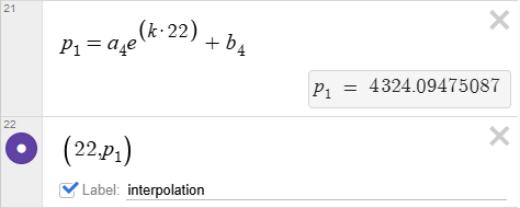
• Extrapolation prediction - choose a distance outside your data range that is larger than your largest measurement, estimate the intensity, plot that point in Desmos, and explain why predictions outside the data range are usually less reliable. Label this point "extrapolation."
• After adjusting the sliders, judging the best fit model, and plotting the interpolation and extrapolation points, click Capture Graph. Paste the graph image into your worksheet.
• When finished, submit your worksheet according to your teacher’s directions.

Going Further:

• Try repeating the above steps to test an interpolated prediction using a different model and compare the results.

Let’s Go:

• Click Hide Directions to give yourself more space. Place the cart 10 cm from the lamp, click Zero Position, then click Start Collection and roll the cart steadily away from the lamp.