What You Will Do:

- Watch the Khan Academy video: "Newton's Law of Cooling"
- Collect temperature data in the Desmos Graphing Calculator for a cup of cooling hot water.
- Use this mathematical model to describe how the temperature of hot water changes over time:
- Observe that the rate of cooling is proportional to the difference in temperature between the hot object and the surrounding room.
- Complete the Google Docs worksheet: "Modeling Newton's Law of Cooling" and turn it in according to your teacher's directions.
$$
f(x) = T_{\text{initial}} - T_{\text{room}}\, e^{\,kx - x_{\text{offset}}} + T_{\text{room}}
$$
- Mathematical Model: a mathematical equation or relationship used to describe, explain, and predict how a real-world system behaves.
- Initial Temperature: the temperature of the hot object at the moment cooling begins.
- Ambient Temperature: the temperature of the surrounding environment that the object is cooling or warming toward.
- Temperature Difference: the difference between the object's temperature and the ambient temperature.
- Cooling Rate Constant: a value that describes how quickly the object cools; larger values mean faster cooling. Physically, this constant depends on the material and environment surrounding the sensor.
- X offset: a horizontal translation of the graph left or right that aligns the model with the moment cooling actually begins.
- Click the Khan Academy video on Newton's Law of Cooling to learn more about these concepts.

- Click this link Temperature - Activity 2 to open the worksheet in a new browser tab. Click 'Make a copy' to save your version to your Google Drive.
- Imagine a hot bowl of soup cooling for some time to room temperature. How would its temperature change as it cools? What would the graph of the cooling curve look like? Use your mouse to click and drag on the graph below to draw your prediction. Click the Erase Drawing if you need to start over.
- When you are satisfied with the drawing, click Capture Drawing to copy the image to the clipboard, then paste it into your Modeling Newton's Law of Cooling Worksheet and answer the related questions.

Directions:
Data Collection:
- Use a USB-C cable to plug the Observe temperature sensor into your computer's USB port.
- Click the Connect button at the top-left corner of this page.
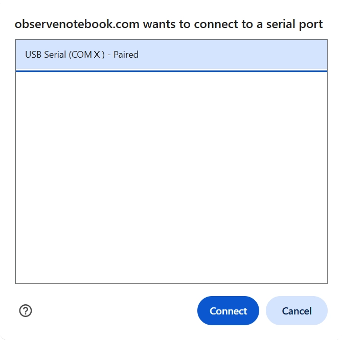
- Select the USB serial port (COM X) and click Connect. X varies by computer and is not important.
- Confirm that the status in the top-right corner says "ready (5 Hz)".
- Set the sensor on the table and do not touch the metal part. Note the temperature shown in the status bar; this is the ambient room temperature. In the Desmos window below, adjust the Troom slider in the expression list to match this value.
- Carefully fill a cup with hot water and place the sensor into it. Note the temperature shown in the status bar; this is the Tinitial. Adjust the Tinitial slider in the expression list to match this value.
- Remove the sensor from the hot water and quickly wipe it dry and click Start Collection to log data as the sensor cools.
- Click Stop Collection after the sensor has cooled to room temperature.
- Clear Graph resets the graph; Zoom to Data fits all collected data within the viewing window; Capture Graph copies the graph; Export / Import saves or opens a CSV data file.
- You may want to clear your graph and repeat a few times until you are satisfied with your data.
- Click the Show Instruction button in the upper-right corner to continue the activity.

- Click the Show Directions in the upper-right corner to learn how to collect temperature data for this activity.
- Select the circle to the left of the mathematical model to display it on the graph. Adjust the model's constant sliders until the model closely fits your data.
- Read the notes in the Desmos expression window. The purpose of this section is to examine how the difference between the hot sensor's temperature and the ambient temperature affects the rate of cooling, the central idea of Newton's Law of Cooling.
- Observe the slope (m) and the coefficient of determination (R2) shown in the linear regression. The slope (m) represents how the rate of cooling changes with temperature difference, while R2 indicates how well a linear model fits the data.
- Compare the slope (m) of the regression with the cooling constant k from the model above. Use this comparison to answer the related questions in your worksheet about whether your data supports Newton's Law of Cooling.
- When finished, click Capture Graph to copy your graph and paste it into your Google Docs worksheet. Be sure your worksheet includes both the graph and your written responses to the analysis questions.
- Collect a second data set, but this time warm the sensor instead of cooling it. Review the steps in the directions.
- Wrap the sensor in a flexible frozen cool-pack and chill it until it drops below zero. Remove the sensor from the cool-pack and click the Start Collection button. Hold the sensor in the air and allow it to warm. Do not touch the metal part. Collect data until the cold sensor warms to room temperature.
- When collection is finished, repeat the steps above in the Analyzing Your Data section.
- When finished, click Capture Graph to copy your graph and paste it into your worksheet.